Attention & Transformers

Posted Dec 20, 2023

By vision-array 9 min read

From Seq-to Seq RNN to Attention & Transformers

This posts address the premise of attention starting from sequence to sequence RNN and builds up all the way to transformer models. These are my notes from the DL4CV course at UMich by Prof. Justin Johnson.

Intro with the time-series data and the Seq-to-Seq

Time Series Data and Long sequences - applications like image captioning, language translation
RNNs types of NN perform better as they have the capability to encode the summary of inputs
One such type of RNN used for language translation is the Seq-to-Seq(Original language sequence to the transalated language sequence)
As the input sentences(sequences) become longer in length - it becomes more diffcult to encode the summary of the input vectors
There is also an initial decoder state given out which is : S0 at the end of the encoder hidden states
Context vector at the end of the encoder summarizes the entire input vectors/sequence information in a lower-dimensional vector
- Longer the input sequence - longer the encoder network - bottleneck on the ability of the context vector to summairze the input better
- higher chance of missing out on key dependencies between inputs like word to word relation in a sentence that might be useful in language translation
The decoder hidden vector at each time step is then related in the following way : $S_t = Gu(S_{t-1}, y_{t-1}, c)$ where “c” is constant and represents the context vector like: $S_1 = Gu(S_0, y_0, c)$

How attention solves the bottleneck of the context vector for longer sequencies ?

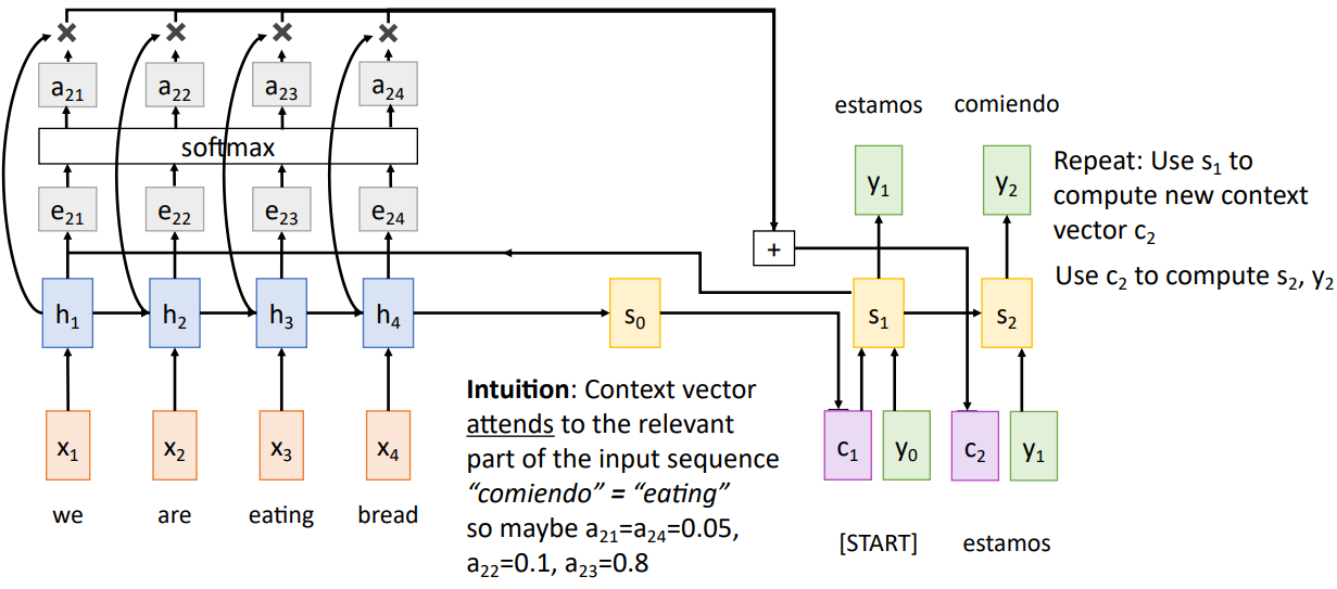
Attention Mechanism allows to learn a context vector for each hidden vector instance of the decoder in such a way that the context vector is calculated as follows
- Alignment scores are calculated for the current decoder hidden vector instance by applying a learnable small MLP network between the previous decoder hidden vector and the concurrent encoder hidden vector
  - $e_{ti} = f_{att}(s_{t-1}, h_i)$ where “i” is for encoder hidden vector and “t” is for the decoder hidden vector
softmax is applied over the attention scores to turn them into probabilities - easier for gradient based optimization and avoiding any singularities - $a_{ti} = Softmax(e_{ti})$
The decoder hidden vector at each time step can then be formulated in the following way : $S_t = Gu(S_{t-1}, y_{t-1}, ct)$ where - $c_t = Sigma_i(a_{ti}, h_i)$
- Implying that the current context vector for the decoder sequence takes in the combined “weighted” summation of the hidden vectors with (the “weights” being the attention weights)
So, this methodology helps focus on different parts of the input sequence/encoder hidden vector for each step of the output/decoder hidden vector through the context vector
This also implies that the decoder doesn’t necessarily consider the encoder hidden vector sequence to be ordered - It just works fine with an unordered sequence too.
We can use this mechanism for Image Captioning - considering that:
- The input/encoder hidden vectors will now be the last feature matrix (last layer of a CNN) of an image.
- The output/decoder hidden vectors will be an RNN for character/word generation.

Generalizing the Attention mechanism into Attention Layer

We then shift focus towards generalizing the attention mechanism into a Layer of a Neural Network

Single Query Vector Case:

Considerations/Assumptions:
- Single Query Vector of Dimension : $q = D_{q}$ (Analogous to the single or current instance of a decoder hidden vector of a decoder of Seq-to-Seq RNN)
- Multiple Input Vector of Dimension : $X = (N_{X}*D_{X})$ – (Analogous to all the encoder hidden vectors of an encoder of Seq-to-Seq RNN)
- Alignment/Attention Score vector of Dimension: $e, a E (N_{X})$
- Output Vector of Dimension: $(Y = D_{X})$ – (Analogous to the current instance of the Context vector of the Seq-to-Seq Decoder RNN)
Alignment scores with the attention function: $e_{i} = f_{att}(q,X_{i})$ can be calculated for the single query vector
Attention score => $a_{i} = Softmax(e_{i})$ for all $i....N_{X}$ of Dimension: $N_{X}$
The output vector is calculated as the weighted sum of attention scores and the inputs $Sigma(a_{i},X_{i})$ (or) a dot product between the similar to the $Sigma(a_{i}, h_{i})$ from the Seq-to-Seq $c_t = Sigma_{i}(a_{ti}, h_{i})$
One way to get the Dimensionality correct with some dot products instead of a $f_{att}$ with an MLP is to use the Input Vectors $(X: (N_{X}*D_{X}))$ to $(N_{X}, D_{q})$, then: we can have a dot product between the Single Query Vector and the Input Vectors as $e_{i} = (q.X_{i})$ where $e = (D_{q}.{(N_{X}*D_{q})}^T) => (D_{q}.(D_{q}*N_{X})) = N_{X}$

Note: Dot Product of two vectors is given by: $A.B = mod(A)mod(B).Cos(theta)$, where mod(A), mod(B) are the vector 2-norms of the two vectors whose value depends on the dimensions of the two vectors, Often in the case of the deep learning context - the query vector and the input vector are long - meaning high dimensional which, so we apply a “scaled-dot-product” where the dot product between the Query vector and the input vector is divided by the $Sqrt(D_{q})$ since vector norm of $$

= q.sqrt(D_{q}) $$

So, the Output vector is still given by the dot product between the attention weight vector of $e E N_{X}$ and the Input Vector $X E (N_{X},D_{X})$
Note: Inorder to get the output vector dimension match with the dimension of the query vector - Select the input vector with the Same Dimensions as $(N_{X}, D_{q})$

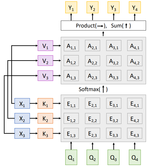
Multiple Query Vector Case:
- Considerations/Assumptions:
  - Query Matrix of Dimension $Q: (N_{Q}*D_{Q})$ - (Analogous to multiple $N_{q}$ instances/multiple steps of a RNN decoder with each decoder hidden vector of dimension $D_{Q}$ )
  - Input Matrix - Multiple Input Vectors of Dimension $X: (N_{X}*D_{Q})$ - (Analogous to the multiple hidden vectors of encoder RNN)
  - Alignment/Attention Scores of Dimension $e E N_{Q}*N_{X}$
  - Output vector of Dimension : $Y E (N_{Q}*D_{Q})$
- The alignment score matrix $e: (N_{Q}*N_{X})$ is calculated using dot product between the Input Matrix and the Query Matrix between the $((N_{Q}*D_{Q}).(N_{X}*D_{Q})^T) = ((N_{Q}*D_{Q})*(D_{Q}*N_{X})) = N_{Q}*N_{X}$ - attention score matrix also with same dimensions $N_{Q}*N_{X}$
- The output vector is calculated as $Sigma(a,N)$ which can also be calculated using the dot product $A.X = ((N_{Q}*N_{X}).(N_{X}*D_{Q}))$ which gives us $Y E N_{Q}*D_{Q}$.
Considering the bifurcation of the input vectors to key and values to introduce the learnable parameters in to weigh how the relevant elements of the input vector should - ( and also consider the dimension of input vector not dependent on the Query Vector dimensions i.e $D_{X}!= D_{Q}$)
- This can be achieved using two different learnable weight matrices:
- $W_{k}$ - Key Weights - Dimensions $(D_{X}*D_{Q})$
- $W_{v}$ - Value Weights - Dimensions $(D_{X}*D_{V})$
- This give us Key Matrix from input vectors as: $K = X.W_{K} = ((N_{X}*D_{X}).(D_{X}*D_{Q})) = (N_{X}*D_{Q})$
- Similarly we get the value matrix from input vectors as: $V = X.W_{v} = ((N_{X}*D_{X}).(D_{X}*D_{Q}))$ which help divide the input vector to key vectors and value vectors
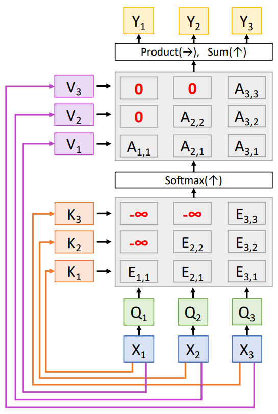
- The alignment scores are then calculated using the key and the Query Matrices as $e = Q.K^T$ , the attention is then calculated as $a = Softmax(e)$ both with the same dimension as $e : Q.K^T = (N_{Q}*D_{Q}).(N_{X}*D_{Q})^T = (N_{Q}*D_{Q}).(D_{Q}*N_{X}) = N_{Q}*N_{X}$,
  - The dot product performed here is again scaled by a factor of $1/(Sqrt(D_{Q}))$ to avoid product of large numbers
  - The Softmax operation for the attention matrix is done across dimension - 1 i.e columns/ across $N_{X}$ Dimension for each of the query vector
- The output is then calculated as the dot product between the $a: (N_{Q}*N_{X})$ attention matrix and the $v: (N_{X}*D_{V})$ value matrix given as $Y = N_{Q}*D_{V}$.

The Self-Attention Layer

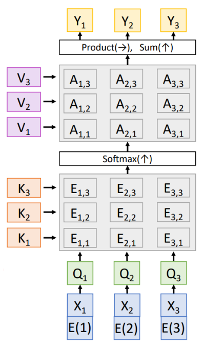
In a self-attention layer - the query vector is also calculated from the input vector using a Learnable Weight matrix for the Query as well
- This implies the number of input vectors is number of query vectors - though the dimensions of each of the individual input vector is different to the dimension of the query vector i.e $N_{X} == N_{Q} and D_{X} != D_{Q}$
- $W_{Q}$ Query Weights matrix is given by - Dimension $(D_{X}*D_{Q})$
- The Query vector is given by $Q: X.W_{Q} = (N_{X}*D_{X})*(D_{X}*D_{Q}) = N_{X}*D_{Q}$
- The rest of the operations on calculating the alignment scores, calculating the attention weights and the output vector is similar to that mentioned above (similar to attention layer) giving the final output vector as $Y = N_{X}*D_{v}$ except that $N_{X} == N_{Q}$
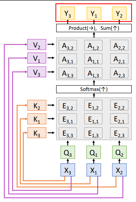
Note: Self-Attention is permutation invariant - i.e the overall output doesnot change except that the output vectors will also be permuted.
- In-order to make the layer position-aware(useful for any time-series data prediction), concatenation of the Positional Encoding done to the input vector.
- The positional encoding could be either a fixed function, a learnable function with a lookup table.
Masked Self-Attention is used when we don’t want the vectors to look ahead in the sequence. (Used in language modeling - predicting next word)
Mulitple-heads can be spinned up in parallel (parallelization for a faster computation) where each handles only some part of the query vector
- Number of Heads and the dimension of the Query Vector become the hyperparameters of the Model at each layer that change the learning ability of the model.
- (in the Attention all you need paper) $D_{Q} = 512 , Num_{Heads} = 8$ giving each split vector of Dimension $D_{Q}/Num_Heads = 64$
- each of the 8 heads are parallely trained on the split input vectors of dimension $N_{X}*64$ and the results can be concatenated along the dimension 1 giving the final output as $N_{X}*512$

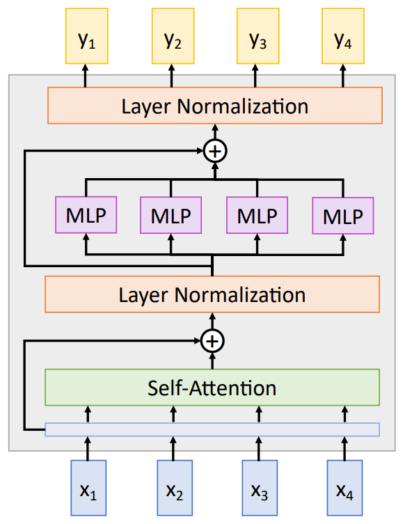
Multiple Self-Attention Layers - Transformer Model

Transformer Models are formed using multiple/repeated blocks, each block consisting of the following layers and operations in the order as stated:
- input to query vectors to Self-Attention layer
- Residual Connection from the input to the output of the Self-Attention Layer
- Layer Normalization
- Individual MLP on each input/query vector
- Concatenating of the output from the with a residual connection from before the individual MLP split
- Layer Normalization - and finally the output vector
  Self-Attention Layer is the only layer where the interaction between the vectors happen The Layer Normalization and the MLP is applied on each input/query Vector indepdent of each other
So:
- The clear advantage is that this is really good for long sequences and for each self-attention layer - the output actually sees all the input vectors and
- It is highly parallelizable.

From the UVA Tutorial

Proper definitions for Tokens, Sequence Length, Dimensionality of the input (Embedded Dimension) => Sequence Length ! = Embdedded Dimension
Head Dimensions for each Q, K , V is (Embdedded Dimension//num_heads) = 512/8 = 64

Reference:

attention, transformers, AI, Deep Learning

attention ML AI deep learning

This post is licensed under CC BY 4.0 by the author.